Python Meets the Fed

The Ultimate Guide to FredAPI

Sep 10, 2024

Did you ever wonder how to easily get free economic data into Python? Look no further – FredAPI is here to revolutionize your quantitative and macroeconomic analysis. In the fast-paced world of financial modeling and economic forecasting, having access to reliable, up-to-date data is not just an advantage – it's a necessity. FredAPI serves as your direct line to the Federal Reserve Economic Data (FRED), a treasure trove of over 816,000 US and international time series from 108 sources.

As quantitative analysts and economists, we often find ourselves juggling multiple data sources, wrestling with inconsistent formats, and spending precious time on data cleaning rather than analysis. FredAPI eliminates these pain points by providing a streamlined, Pythonic interface to access a vast array of economic indicators. Whether you're building predictive models, back-testing trading strategies, or conducting in-depth economic research, FredAPI empowers you to focus on what truly matters – deriving insights from the data.

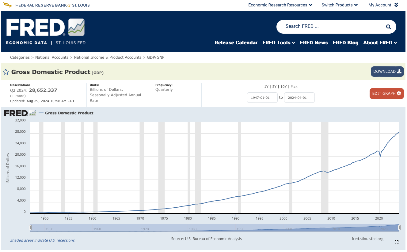
Source: https://fred.stlouisfed.org/series/GDP

In this comprehensive guide, we'll explore how FredAPI can supercharge your quantitative toolkit. From basic data retrieval to creating complex, multi-variable dashboards, you'll learn how to leverage this powerful library to its fullest potential. By the end of this journey, you'll be equipped to effortlessly integrate real-time economic data into your Python workflows, giving you a competitive edge in the world of quantitative finance and macroeconomic analysis. So, are you ready to unlock the full potential of economic data in your Python projects? Let's dive in!

Initial Setup: Installing and Configuring FredAPI

Before we begin our data exploration, let's set up our environment. First, install FredAPI:

pip install fredapi

Once installed, import the library and configure your API key:

import fredapi as fa
fred = fa.Fred(api_key='your_api_key_here')

Replace 'your_api_key_here' with your actual API key from the FRED website. This key is your access point to a vast repository of economic data, so ensure it's kept secure.

Basic Data Retrieval: Fetching Unemployment Data

Let's start with a fundamental economic indicator: the unemployment rate. This metric is crucial for assessing overall economic health and is often a key input for macroeconomic models.

To retrieve this data, we use the fred.get_series() function, the primary method for data extraction in FredAPI. This function requires a 'series_id' as its main argument. You can find these series IDs on the FRED website or by using FredAPI's search functionality.

import pandas as pd

unemployment = fred.get_series('UNRATE')

pd.DataFrame(unemployment, columns=['Unemployment_Rate']).tail()

By default, this retrieves the entire available history of the unemployment rate. Having this long-term perspective can be invaluable for many analyses, allowing you to identify trends and cycles over extended periods.

Specifying Date Ranges: Analyzing Production Data

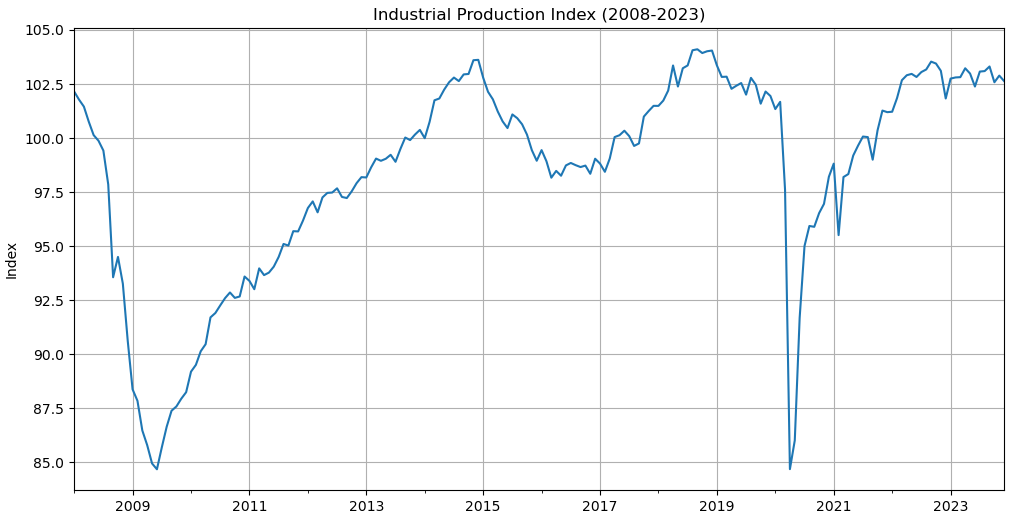
Often, your analysis may focus on a specific time period. For instance, if we're examining the production performance since the 2008 financial crisis, we can use the Industrial Production Index and specify a date range:

import matplotlib.pyplot as plt

industrial_production = fred.get_series('indpro', 
                                    observation_start='2008-01-01', 
                                    observation_end='2023-12-31')

industrial_production.plot(figsize=(12, 6))
plt.title('Industrial Production Index (2008-2023)')
plt.ylabel('Index')
plt.grid(True)
plt.show()

The observation_start and observation_end parameters allow us to focus on specific periods. This functionality is particularly useful when studying the effects of certain events or policies, or when you want to exclude unusual periods that might skew your analysis.

Adjusting Data Frequency: Examining the Federal Funds Rate

Different analyses require different data granularities. Let's examine the Federal Funds Rate, a key monetary policy tool, and demonstrate how to adjust its frequency:

fed_rate_monthly = fred.get_series('FEDFUNDS', frequency='m')
fed_rate_quarterly = fred.get_series('FEDFUNDS', frequency='q')
fed_rate_annual = fred.get_series('FEDFUNDS', frequency='a')

fig, (ax1, ax2, ax3) = plt.subplots(3, 1, figsize=(12, 15))
fed_rate_monthly['2020':].plot(ax=ax1, title='Monthly Fed Funds Rate')
fed_rate_quarterly['2020':].plot(ax=ax2, title='Quarterly Fed Funds Rate')
fed_rate_annual['2000':].plot(ax=ax3, title='Annual Fed Funds Rate')
plt.tight_layout()
plt.show()

The frequency parameter allows you to specify the time scale of your data. Use 'd' for daily, 'w' for weekly, 'm' for monthly, 'q' for quarterly, or 'a' for annual data. This flexibility is crucial because different economic indicators have different natural frequencies, and your models might require specific time scales.

For instance, if you're building a model to predict quarterly GDP growth, you might want to align all your input variables to a quarterly frequency. Conversely, for long-term trend analysis, annual data might suffice and could smooth out short-term fluctuations.

Data Transformations: Analyzing CPI Data

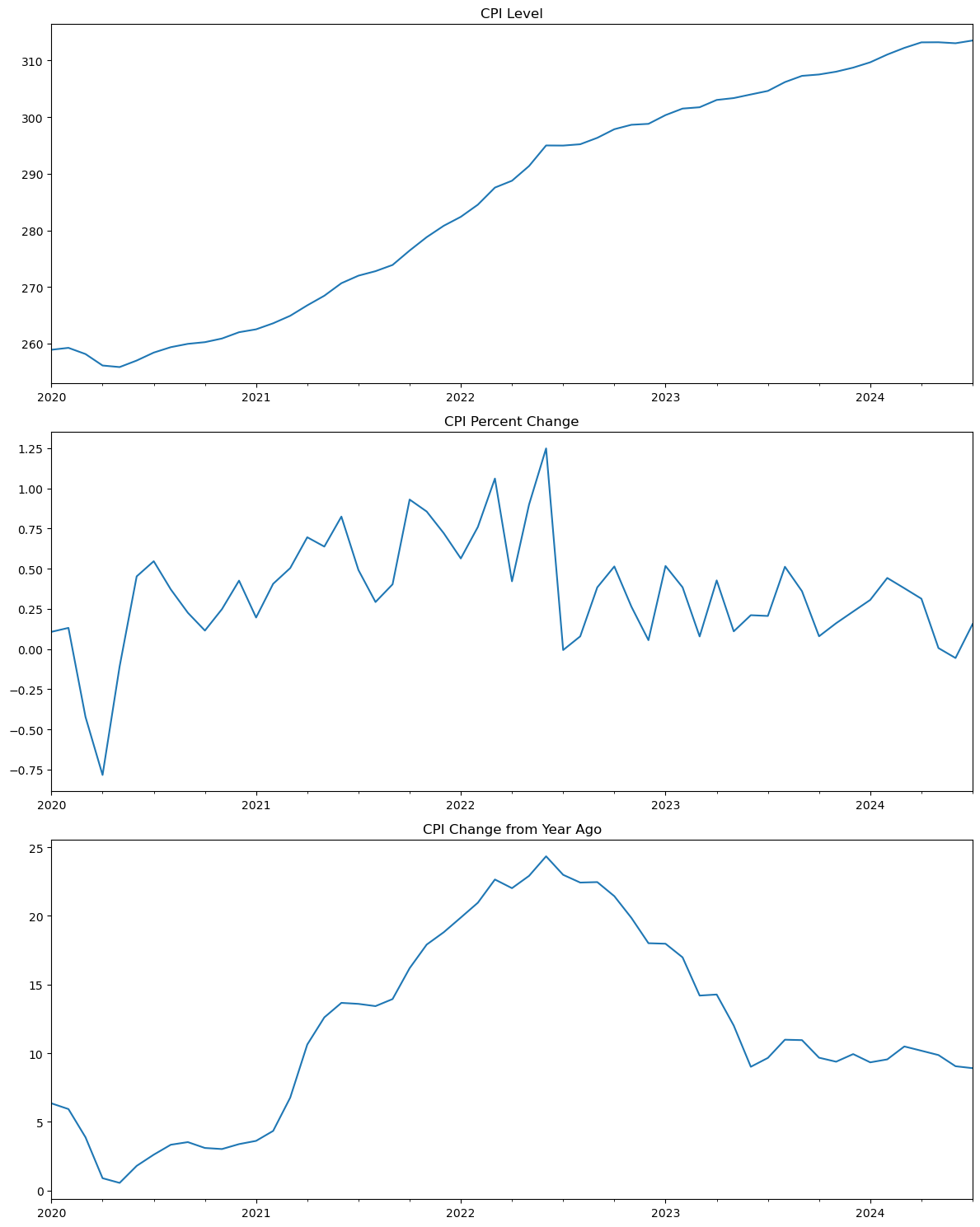
In many cases, we need to view data from different perspectives. The Consumer Price Index (CPI) serves as an excellent example. We might need to analyze its absolute level, its percentage change, or its change from a year ago. FredAPI's units parameter facilitates these transformations:

cpi_level = fred.get_series('CPIAUCSL', units='lin')  # Linear (level)
cpi_pct_change = fred.get_series('CPIAUCSL', units='pch')  # Percent change
cpi_chg_year_ago = fred.get_series('CPIAUCSL', units='ch1')  # Change from year ago

fig, (ax1, ax2, ax3) = plt.subplots(3, 1, figsize=(12, 15))
cpi_level['2020':].plot(ax=ax1, title='CPI Level')
cpi_pct_change['2020':].plot(ax=ax2, title='CPI Percent Change')
cpi_chg_year_ago['2020':].plot(ax=ax3, title='CPI Change from Year Ago')
plt.tight_layout()
plt.show()

The units parameter offers various transformation options:

'lin': Linear (no transformation)
'chg': Change
'ch1': Change from a year ago
'pch': Percent change
'pc1': Percent change from a year ago
'pca': Compounded annual rate of change
'cch': Continuously compounded rate of change
'cca': Continuously compounded annual rate of change
'log': Natural log

These transformations are essential for various analyses. For example, when examining inflation, economists often focus on year-over-year percent changes rather than absolute levels.

Comprehensive Analysis: Creating a MacroQuant Dashboard

Now that we've explored various aspects of FredAPI, let's integrate our knowledge to create a comprehensive macroeconomic dashboard:

import pandas as pd
import seaborn as sns
import matplotlib.pyplot as plt

def fetch_macro_data(start_date='2000-01-01'):
    return pd.DataFrame({
        'Unemployment': fred.get_series('UNRATE', observation_start=start_date, frequency='q'),
        'Industrial Production': fred.get_series('indpro', observation_start=start_date, frequency='q'),
        'Fed Funds Rate': fred.get_series('FEDFUNDS', observation_start=start_date, frequency='q'),
        'CPI': fred.get_series('CPIAUCSL', observation_start=start_date, frequency='q', units='pch'),
        'GDP Growth': fred.get_series('GDP', observation_start=start_date, frequency='q', units='pch'),
        'Yield Curve': fred.get_series('T10Y2Y', observation_start=start_date, frequency='q'),
    })

macro_data = fetch_macro_data()

# Set up the matplotlib figure
fig, axes = plt.subplots(3, 2, figsize=(20, 20))
fig.suptitle('MacroQuant Economic Dashboard', fontsize=16)

# Plot each indicator
for (col, ax) in zip(macro_data.columns, axes.flatten()):
    sns.lineplot(data=macro_data, x=macro_data.index, y=col, ax=ax)
    ax.set_title(col)
    ax.grid(True)

# Adjust layout and display
plt.tight_layout()
plt.show()

This dashboard consolidates several key economic indicators, each retrieved and transformed according to our specific requirements. We're using quarterly data for consistency, but you could easily adjust this based on your analysis needs.

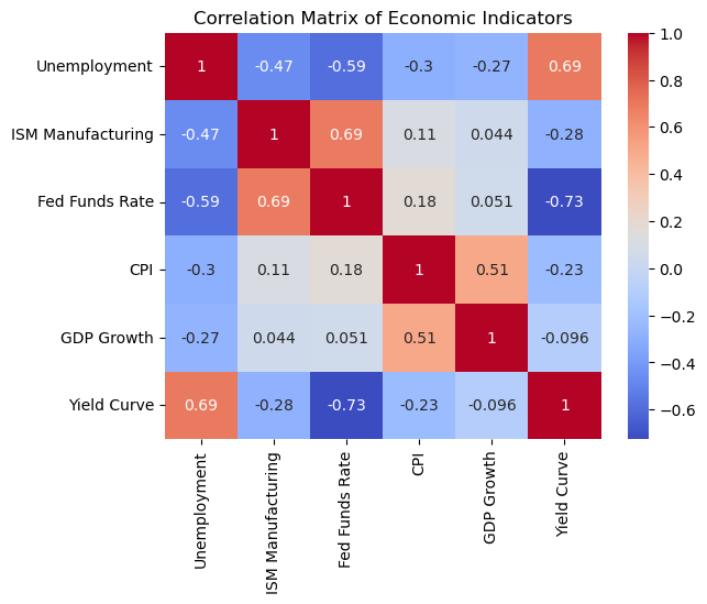
# Print correlation matrix
sns.heatmap(macro_data.corr(), annot=True, cmap='coolwarm')
plt.title('Correlation Matrix of Economic Indicators')
plt.show()

The correlation heatmap provides a quick visualization of relationships between different economic variables, which can be an excellent starting point for developing hypotheses or identifying potential leading indicators for your models.

Conclusion

FredAPI is a powerful tool for quantitative researchers and macroeconomic analysts. Its seamless Python integration allows for easy incorporation of a wide range of economic data into your analytical workflows. From basic data retrieval to building comprehensive dashboards, FredAPI provides the tools you need to enhance your macroquant models with robust, up-to-date economic indicators.

At MacroQuant Insights, we're committed to equipping you with cutting-edge tools for portfolio construction and macroeconomic analysis. FredAPI is an essential addition to your quantitative toolkit, enabling you to stay current with economic trends and make data-driven decisions.

Disclaimer:

The content provided on MacroQuant Insights is for informational and educational purposes only and should not be construed as financial advice. While we strive to provide accurate and timely information, all data and analysis are based on sources believed to be reliable but are not guaranteed for accuracy, reliability, or completeness. The opinions expressed are solely those of the author and do not constitute endorsements or recommendations for any specific investment strategy, security, or action.

Investing involves risk, including the potential loss of principal. Past performance is not indicative of future results. Always conduct your own research and consult with a qualified financial advisor or other professional before making any investment decisions. MacroQuant Insights and its contributors disclaim all liability for any investment decisions made based on the information provided, and no warranty is made as to the accuracy or completeness of the information presented.

Remember, all investments carry risks, and it is important to fully understand these risks before acting on any information presented on this blog. Users are solely responsible for their own investment decisions. MacroQuant Insights is not responsible for any outcomes resulting from the use of this information, and all content is subject to change without notice.

MacroQuant Insights